-
Notifications
You must be signed in to change notification settings - Fork 141
Segmentation
We describe how to segment our anatomical images into different tissue types. We are frequently interested in identifying the grey matter so that we restrict fMRI analysis. We are also interested in the gray-white boundary which can be used to create the representation of the cortical surface we use for visualizations. Finally, we are interested in white matter to control the tractography.
We use [Freesurfer's](http://surfer.nmr.mgh.harvard.edu/fswiki) automated segmentation procedure to create the labels (and other files). This is a useful tool. In some cases we perform additional hand editing using [ITKSnap](http://www.itksnap.org/pmwiki/pmwiki.php).
_Note: Michael Perry has implemented a docker container that executes Freesurfer. This will be run automatically when we start to rely on the Flywheel scientific data management tool. In the mean time, the instructions below will guide the manual approach._
To run Freesurfer routinely it is best to include some lines in your resource file that identify key directories. For example the .bashrc file, typically in your home directory and executed at login, might contain the following lines
    export SUBJECTS_DIR=/biac2/kgs/3Danat/FreesurferSegmentations > /dev/null
    export FREESURFER_HOME=/white/local/freesurfer/v5.1.0 > /dev/null
    source $FREESURFER_HOME/SetUpFreeSurfer.sh > /dev/null
These define the directory where Freesurfer segmentations end up as well as the location of our Freesurfer code, and then executes a command to setup Freesurfer in your shell.
In some situations the resource file is not automatically executed. You can run it from the command line,
source ~/.bashrc
Here are a few lines of code in MATLAB that will:
1. create a Freesurfer segmentation (ribbon.mgz file) from a T1 nifti using the Freesurfer command recon-all 2. transform the ribbon.mgz file into a Vistasoft class file for use in mrVista.
We generally average our T1 anatomies and AC-PC align them before doing this step [AC-PCalignment](https://github.com/vistalab/vistasoft/wiki/ACPC%20alignment). It is also a good idea (at least for Stanford CNI data) to use the command niftiApplyCanonicalXform on your average T1.
%% script that will call freesurfer command and convert the ribbon file into a nifti class file. % first we create a subjectID. Freesurfer will use this to name the directory where it puts its output files. % so in this case it will be
subjectID = '';
% it is generally helpful to make the subjectID the same as the name of the mrVista Session % next we need the path where freesurfer will put the directory. if you don't know the path you can get it by typing % echo $SUBJECTS_DIR in a terminal window
dirFS = '/biac2/kgs/3Danat/FreesurferSegmentations/';
% then we set the path to the subject's anatomy directory. This is where the subject's T1 is and where the classFile % will be made. As a note, Freesurfer seems to like full paths and not relative ones.
dirAnat = '';
% then the name of our t1 file
pathT1 = 't1average.nii.gz';
% this is the path to the ribbon file that will be made by Freesurfer
inputRibbonFile = fullfile(dirFSsubject, 'mri','ribbon.mgz');
% then where we will save the class file created from ribbon.mgz
outputClassNii = fullfile(dirAnat, 't1_class_pretouchup.nii.gz');
% run Freesurfer
eval(['! recon-all -i ' pathT1 ' -subjid ' dirNameFreesurfer ' -all'])
% once Freesurfer is finished we convert the ribbon file to mrVista class file
fs_ribbon2itk(, , [], ) fs_ribbon2itk(inputRibbonFile, outputClassNii, [], pathT1, [])
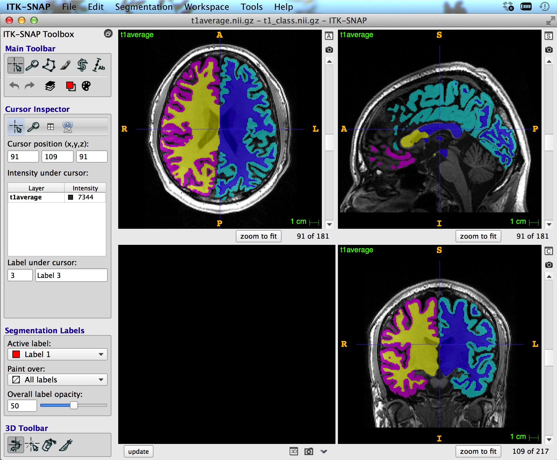
Checking the Segmentation in [itkSnap](http://www.itksnap.org/pmwiki/pmwiki.php)
(1) Open t1 in itkSnap
Open the itkSnap app from the finder window. In the window that pops up, select "Open Image" and then select the t1.nii.gz file you just created. Click "Next" and then "Finish."
This will open the itkSnap GUI, made up of four windows: three showing the axial, coronal, and sagittal views.

(2) Load the segmentation (class) file.
From the menu bar, select Segmentation --> Open Segmentation. Select the t1_class.nii.gz file. This should overlay the segmentation on your anatomical image.

(2) Inspect each hemisphere
First, turn off all the labels except the gray and white matter labels from the hemisphere you are inspecting. You can do this by clicking on the icon in the main toolbar (top left) that looks like a painter's pallet. Or alternatively, from the menu bar select Segmentation/labeleditor
Scroll through the slices in each of the three windows using either the arrow keys or the mouse wheel. Check that the white matter label generally only covers the white matter, and that the gray matter is of reasonable thickness (couple mm).
Check the 3D mesh. In the 3D window (bottom left), click 'update' to see the 3D mesh.

Annoyingly, sometimes the labels that you turned off show up here. If that's the case, open the label editor and set the unwanted labels' opacity to 0.
Inspect mesh for holes, strange protrusions, and areas where white matter pokes through the gray matter
(3) Consider manually editing mesh
The autosegmentation is frequently used as is. Sometimes, however, it makes mistakes particularly around the occipital pole. You may wish to manually edit the segmentation; this process is time consuming and painful. Instructions and guidelines can be found here.
- Vistasoft
- Getting Started
- mrVista Overview
- Anatomy
- Functional MRI
- mrVista
- Retinotopy tutorial
- Population RF methods also prf Model, prf_tutorial, prf tutorial
- Diffusion weighted MRI
- Visualization
- Tractography
- Tutorials
- Software overview