Runge-Kutta integrating factor (IF) and exponential time-differencing (ETD) methods
for solving nonlinear-PDE's of the form ut = Lu + NL(u).
Some examples of non-linear PDES that can be numerically solved using these methods are:
- Nonlinear Schrodinger equation (NLS)
- Kuramoto-Sivashinsky (KS)
- Korteweg-de Vries (KdV)
- Burgers
- Allen-Cahn
- Sine-Gordon
The adaptive step solver options provided in this package are
- ETD35 (5th order ETD with 3rd orderembedding)
- ETD34 (4th order ETD with 3rd order embedding)
- IF34 (4th order IF with 3rd order embedding)
- IF45DP (5th order IF with 4th order embedding)
The constant step solver options provided are
- ETD4 (4th order ETD - Krogstad method)
- ETD5 (5th order ETD - same as the 5th order method in ETD35)
- IF4 (4th order IF - same as the 4th order method in IF34)
In general, one should prefer ETD35 as it often has the best speed and stability for diagonal systems or diagonalized non-diagonal systems. Because the RK coefficients can be costly to compute, IF34 or constant step methods may be preferable in certain settings. A detailed discussion of these solvers is provided in the journal article Exponential time-differencing with embedded Runge–Kutta adaptive step control .
Package requires
- numpy
- scipy
- numpy = 1.19.2
- scipy = 1.6.0
Each of the solvers is a python class (UPPERCASE) stored in a module of the same name (lowercase). Initializing each class requires two arguments, a linear operator L in the form of a numpy array, and a nonlinear function NL(u). The solvers can then be proagated either by using the solver.step function (user steps through time) or using the solver.evolve function (stepping handled internally). For example
from rkstiff import etd35
L = # some linear operator
def NL(u): #  nonlinear function defined here
solver = etd35.ETD35(linop=L,NLfunc=NL)
u0 = # initial field to be propagated
t0 =  # initial time
tf = # final time
uf = solver.evolve(u0,t0=t0,tf=tf)
By default, when using the function evolve, the field is stored at each step in a python list: u0,u1,...,uf are stored in solver.u. The corresponding times t0,t1,...,tf are stored in solver.t.
Consider the Kuramoto-Sivashinsky (KS) equation:
ut = -uxx - uxxxx - uux.
Converting to spectral space using a Fourier transform (F) we have
vt = kx2(1- kx2)v - F { F-1 {v} F-1{ i kx v} }
where v = F{u}. We can then plug L = kx2(1- kx2), and NL(u) = - F { F-1 {v} F-1{ i kx v} } into an rkstiff solver and propagate the field u in spectral space, converting back to real space when desired. For exampe, the python code may look something like this
import numpy as np
from rkstiff import grids
from rkstiff import if34

# uniform grid spacing, real-valued u -> construct_x_kx_rfft
N = 8192
a,b = 0,32*np.pi
x,kx = grids.construct_x_kx_rfft(N,a,b)

L = kx**2*(1-kx**2)
def NL(uFFT):
    u = np.fft.irfft(uFFT)
    ux = np.fft.irfft(1j*kx*uFFT)
    return -np.fft.rfft(u*ux)

u0 = np.cos(x/16)*(1.+np.sin(x/16))
u0FFT = np.fft.rfft(u0)
solver = if34.IF34(linop=L,NLfunc=NL)
ufFFT = solver.evolve(u0FFT,t0=0,tf=50,store_freq=20) # store every 20th step in solver.u and solver.t
U = []
for uFFT in solver.u:
    U.append(np.fft.irfft(uFFT))
U = np.array(U)
t = np.array(solver.t)
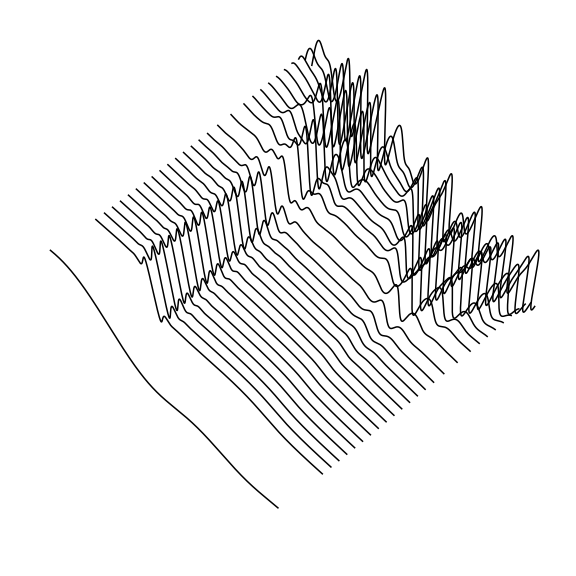
The grid module in rkstiff has several useful helper functions for setting up spatial and spectral grids. Here we used it to construct grids for a real-valued u utilizing the real-valued numpy Fourier transform (rfft). The results of the KS 'chaotic' propagation are shown below.
From the github source
git clone https://github.com/whalenpt/rkstiff.git
cd rkstiff
python3 -m pip install .
PyPI install with a virtualenv (see the Python Packaging Authority guide)
python3 -m venv env
source env/bin/activate
python3 -m pip install rkstiff
For use with Anaconda using the conda-forge channel (see the Getting started with conda guide), from the terminal
conda create --name rkstiff-env
conda activate rkstiff-env
conda install rkstiff -c conda-forge
The demos require installation of the python matplotlib and jupyter packages in addition to numpy and scipy. The tests require installation of the python package pytest. These may be installed seperately or by using
python3 -m pip install '.[demo]'
python3 -m pip install '.[test]'
when installing from the rkstiff source directory
This project is licensed under the MIT License - see the LICENSE file for details.
@article{WHALEN2015579,
title = {Exponential time-differencing with embedded Runge–Kutta adaptive step control},
journal = {Journal of Computational Physics},
volume = {280},
pages = {579-601},
year = {2015},
author = {P. Whalen and M. Brio and J.V. Moloney}
}
Patrick Whalen - whalenpt@gmail.com

