MaAsLin2 is the next generation of MaAsLin (Microbiome Multivariable Association with Linear Models).
MaAsLin2 is a comprehensive R package for efficiently determining multivariable association between clinical metadata and microbial meta-omics features. MaAsLin2 relies on general linear models to accommodate most modern epidemiological study designs, including cross-sectional and longitudinal, along with a variety of data exploration, normalization, and transformation methods.
If you use the MaAsLin2 software, please cite our manuscript: Himel Mallick, Timothy L. Tickle, Lauren J. McIver, Gholamali Rahnavard, Long H. Nguyen, George Weingart, Siyuan Ma, Boyu Ren, Emma Schwager, Ayshwarya Subramanian, Joseph N. Paulson, Eric A. Franzosa, Hector Corrada Bravo, Curtis Huttenhower. "Multivariable Association in Population-scale Meta-omics Studies" (In Submission).
If you have questions, please direct it to :
MaAsLin2 Forum
Google Groups (Read only)
- 1. Introduction to R
- 2. Installing MaAsLin2
- 3. Microbiome Association Detection with MaAsLin2
- 4. Advanced Topics
- 5. Command Line Interface
R is a programming language specializing in statistical computing and graphics. You can use R just the same as any other programming languages, but it is most useful for statistical analyses, with well-established packages for common tasks such as linear modeling, 'omic data analysis, machine learning, and visualization.
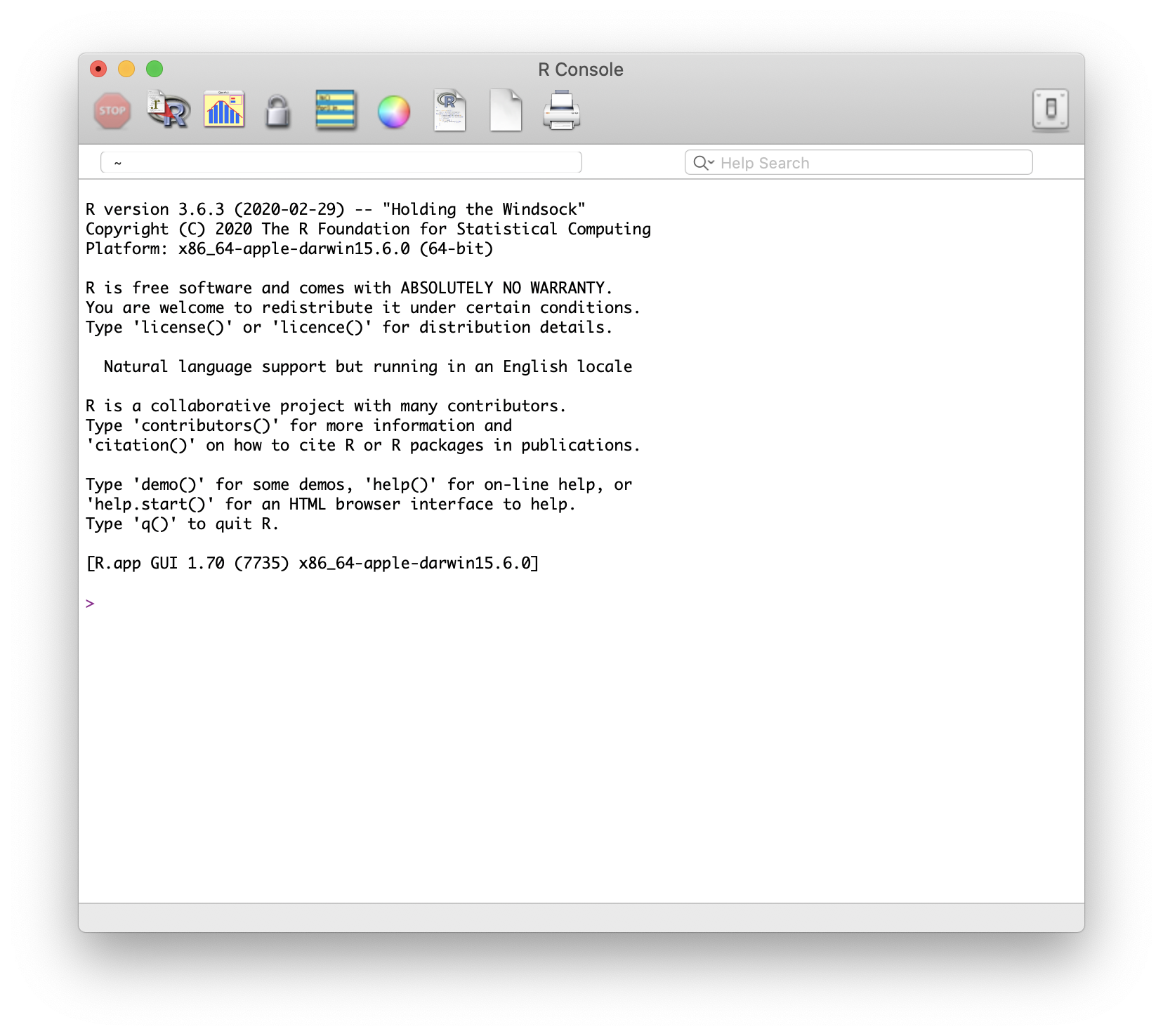
You can download and install the free R software environment here. Note that you should download the latest release - this will ensure the R version you have is compatible with MaAsLin2. Once you've finished the installation, locate the R software and launch it - you should have a window that looks like this:
RStudio is a freely available IDE (integrated development environment) for R. It is a "wrapper" around R with some additional functionalities that makes programming in R a bit easier. Feel free to download RStudio and explore its interface - but it is not required for this tutorial.
If you already have R installed, then it is possible that the R version you have
does not support MaAsLin2. The easiest way to check this is to launch R/RStudio,
and in the console ("Console" pane in RStudio), type in the following command
(without the > symbol):
> sessionInfo()
The first line of output message should indicate your current R version. For example, I got
> sessionInfo()
R version 3.6.3 (2020-02-29)
For MaAsLin2 to install, you will need R >= 3.6.0. If your version is older than
that, please refer to section
Installing R for the first time to download
the latest R. Note that
RStudio users will need to have RStudio "switch" to this later version once it
is installed. This should happen automatically for Windows and Mac OS users when
you relaunch RStudio. For Linux users you might need to bind the correct R
executable. For more information refer to here. Either way, once you have the correct version installed, launch
the software and use sessionInfo() to make sure that you indeed have R >= 3.6.0.
The user interacts with R by inputting commands at the prompt (>). We did so above
by using the sessionInf() command. We can also, for example, ask R to do basic
cacluations for us:
> 1 + 1
[1] 2
Additional operators include -, *, /, and ^ (exponentiation). As an
example, the following command caculates the (approximate) area of a circle with
a radius of 2:
> 3.14 * 2^2
[1] 12.56
You can create variables in R - individual units with names to store values in. These units can then be called on later on, to examine or use their stored values:
> r = 2
In the above command, I created a variable named r, and assigned the value 2
to it (using the = operator). Note that the above command didn't prompt R to
generate any output messages; the operation here is implicit. However, I can now
call on r to check its stored value:
> r
[1] 2
I can use stored variables for future operations:
> 3.14 * r^2
[1] 12.56
R has some built-in variables that we can directly make use of. For example, the
pi variable stores a more accurate version of the constant 3.14:
> pi
[1] 3.141593
Now, can you make sense of the following operations (notice how I can change the
value stored in r with a new assignment operation):
> r = 3
> area = pi * r^2
> area
[1] 28.27433
Lastly, R can use and handle other "classes" of values than just numbers. For example, character strings:
> circle = "cake"
> circle
[1] "cake"
- Question: try the following command in R:
circle = cake
Does it run succesfully? What is the problem?
Functions are conveniently enclosed operations, that take zero or more input
and generate the desired outcome. We use a couple of examples to illustrate the
concept of R functions. The first one, the very basic c() function, combines
values into a vector:
> c(1, 2, 3)
[1] 1 2 3
Notice that you call functions by providing parameters (values in the the parentheses) as input. They then (most times) return values as input. You can, of course, use variables as input, or assign the returned value to new variables. Imagine two researchers individually collected sample measurements of the same population, and now would like to combine their data. They can do so with:
> samples1 = c(3, 4, 2, 4, 7, 5, 5, 6, 3, 2)
> samples2 = c(2, 3)
> samples_all = c(samples1, samples2)
> samples_all
 [1] 3 4 2 4 7 5 5 6 3 2 2 3
The second example, t.test(), does exactly what its name suggests: it performs
a t-test between two vectors,
to see if the difference in their means is statistically significant:
> t.test(samples1, samples2)

	Welch Two Sample t-test

data:  samples1 and samples2
t = 2.2047, df = 3.9065, p-value = 0.09379
alternative hypothesis: true difference in means is not equal to 0
95 percent confidence interval:
 -0.4340879  3.6340879
sample estimates:
mean of x mean of y
      4.1       2.5
Certain function parameters have names, and you can explicitly invoke them during
function calls. For example, here you will notice that the test performed
is a two-sided test.
What if we wanted to perform a one-sided test, to see if the average of samples1 is
significantly higher than that of samples2? For this, we can invoke the
alternative parameter in t.test(), which lets us select one of the options
("two.sided", "less", or "greater"), depending on the alternative hypothesis
we are interested in.
> t.test(x = samples1, y = samples2, alternative = "greater")

	Welch Two Sample t-test

data:  samples1 and samples2
t = 2.2047, df = 3.9065, p-value = 0.04689
alternative hypothesis: true difference in means is greater than 0
95 percent confidence interval:
 0.04217443        Inf
sample estimates:
mean of x mean of y
      4.1       2.5
You can check the full list of parameters for functions in R with the command
? + function name. For example ?t.test gives you the full documentation
for the function t.test.
The functions we used so far are built-in. Just like variables, we can also
create our own functions, by involking the function keyword.
> area_circle = function(r) {
     return(pi * r^2)
  }
> area_circle(r = 3)
[1] 28.27433
- Question: study the following two functions, aimed at calculating the overall
mean of samples collected by two separate researchers.
- What happened in each function?
- What are their differences?
- Which one is better?
> overall_mean1 = function(samples1, samples2) {
      samples_all = c(samples1, samples2)
      return(mean(samples_all))
  }
> overall_mean2 = function(samples1, samples2) {
      mean1 = mean(samples1)
      mean2 = mean(samples2)
      return((mean1 + mean2) / 2)
  }
- Hint: imagine the following scenarios:
- If the first researcher collected a lot more samples than the second one, which way is better?
- If the first researcher collected a lot more samples than the second one, but their experimetal protocal is flawed, leading to overestimation of measurements, which way is better?
Once you have the correct R version, you can install MaAsLin2 with Bioconductor:
if(!requireNamespace("BiocManager", quietly = TRUE))
    install.packages("BiocManager")
BiocManager::install("Maaslin2")
You might encounter an error message that states:
Warning message:
package ‘Maaslin2’ is not available (for R version x.x.x)
This can be due to one of two reasons:
-
Your R version is too old. Check this with
sessionInfo()- if it is older than 3.6, download the most updated version per instructions above. -
You have an older version of Bioconductor. MaAsLin2 requires Bioconductor >= 3.10. You can check your Bioconductor version with
BiocManager::version(). If the returned version is anything older than 3.10, you can update with
BiocManager::install(version = "3.10)
And then
BiocManager::install("Maaslin2")
This is a place holder right now.
MaAsLin2 requires two input files, one for taxonomic or functional feature abundances, and one for sample metadata.
- Data (or features) file
- This file is tab-delimited.
- Formatted with features as columns and samples as rows.
- The transpose of this format is also okay.
- Possible features in this file include taxonomy or genes.
- Metadata file
- This file is tab-delimited.
- Formatted with features as columns and samples as rows.
- The transpose of this format is also okay.
The data file can contain samples not included in the metadata file (along with the reverse case). For both cases, those samples not included in both files will be removed from the analysis. Also the samples do not need to be in the same order in the two files.
Example input files can be found in the inst/extdata folder
of the MaAsLin2 source. The files provided were generated from
the HMP2 data which can be downloaded from https://ibdmdb.org/ .
input_data = system.file(
    "extdata", "HMP2_taxonomy.tsv", package="Maaslin2") # The abundance table file
input_data
input_metadata = system.file(
    "extdata", "HMP2_metadata.tsv", package="Maaslin2") # The metadata table file
input_metadata
HMP2_taxonomy.tsv: is a tab-demilited file with species as columns and
samples as rows. It is a subset of the taxonomy file so it just includes the
species abundances for all samples.
HMP2_metadata.tsv: is a tab-delimited file with samples as rows and metadata
as columns. It is a subset of the metadata file so that it just includes some of
the fields.
The following command runs MaAsLin2 on the HMP2 data, running a multivariable
regression model to test for the association between microbial species abundance
versus IBD diagnosis and dysbiosis scores
(fixed_effects = c("diagnosis", "dysbiosis")). Output are generated in a
folder called demo_output under my home directory (output = "~/demo_output").
library(Maaslin2) ## This loads MaAsLin2 into your R environment
fit_data = Maaslin2(
    input_data = input_data,
    input_metadata = input_metadata,
    output = "~/demo_output",
    fixed_effects = c("diagnosis", "dysbiosis"))
If you are familiar with the data frame class in R, you can also provide data
frames for input_data and input_metadata for MaAsLin2, instead of
file names. One potential benefit of this approach is that it allows you to
easily manipulate these input data within the R enviroment.
df_input_data = read.table(file = input_data, header = TRUE, sep = "\t",
                            row.names = 1,
                            stringsAsFactors = FALSE)
df_input_data[1:5, 1:5]
df_input_metadata = read.table(file = input_metadata, header = TRUE, sep = "\t",
                                row.names = 1,
                                stringsAsFactors = FALSE)
df_input_metadata[1:5, ]
fit_data2 = Maaslin2(
    input_data = df_input_data,
    input_metadata = df_input_metadata,
    output = "~/demo_output2",
    fixed_effects = c("diagnosis", "dysbiosis"))
- Question: how would I run the same analysis, but only on CD and nonIBD
subjects?
- Hint: try
?subset
- Hint: try
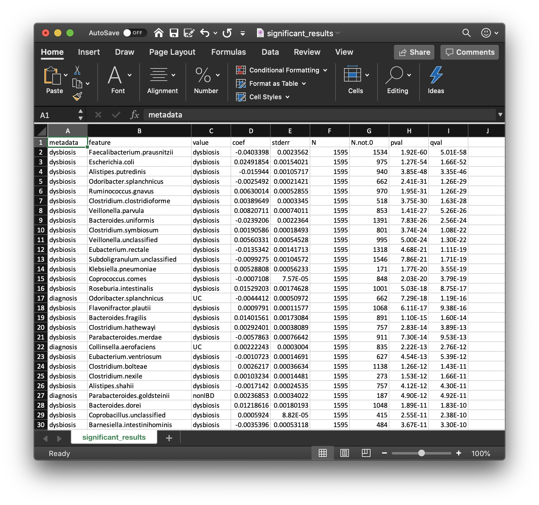
Perhaps the most important output from MaAsLin2 is the list of significant
associations. These are provided in significant_results.tsv:
These are the full list of associations that pass MaAsLin2's significance threshold, ordered by increasing q-values. Columns are:
-
The first columns are the metadata and feature names.
-
The next two columns are the value and coefficient from the model.
- Coefficients for categorical variables indicate the contrast between the
category specified in
valueversus the reference category. - MaAsLin2 by default sets the first category in alphabetical order as the reference. See 4.1 Setting Reference Levels on how to change this behavior.
- Coefficients for categorical variables indicate the contrast between the
category specified in
-
The next column is the standard deviation from the model.
-
The
Ncolumn is the total number of data points. -
The
N.not.zerocolumn is the total of non-zero data points. -
The pvalue from the calculation is the second to last column.
-
The qvalue is computed with
p.adjustwith the correction method. -
Question: how would you interpret the first row of this table?
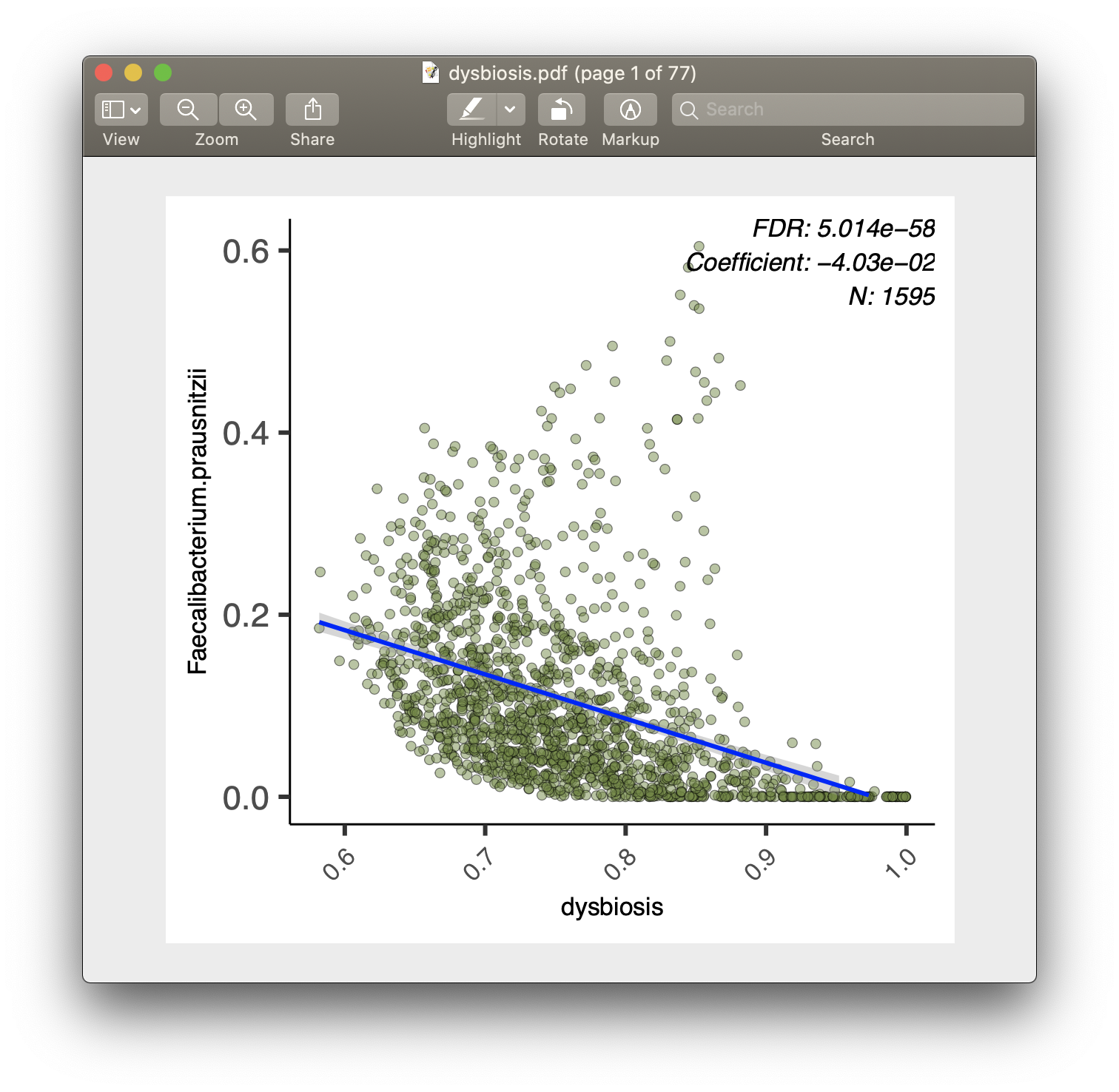
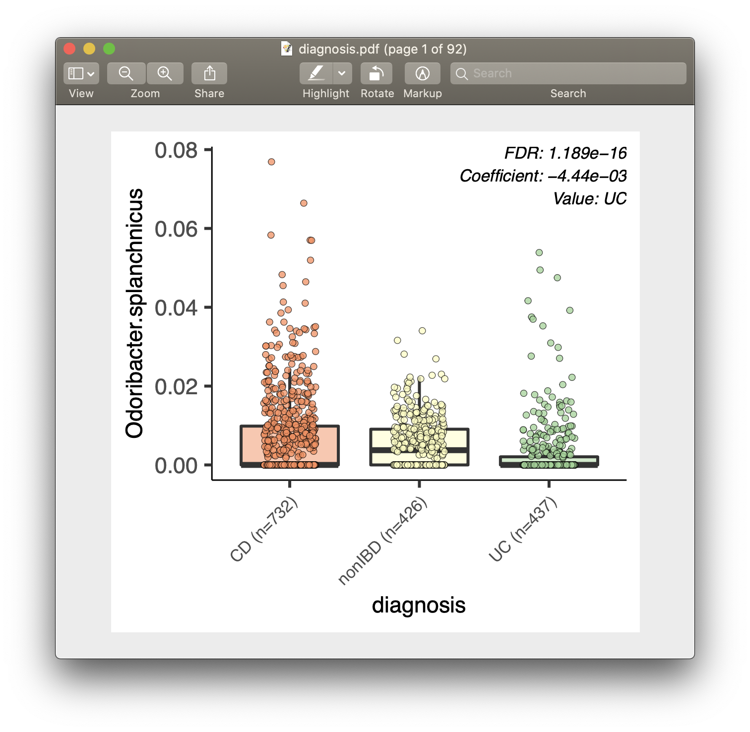
For each of the significant associations in significant_results.tsv, MaAsLin2
also generates visualizations for inspection (boxplots for categorical variables,
scatter plots for continuous). These are named as "metadata_name.pdf". For
example, from our analysis run, we have the visualization files dysbiosis.pdf
and diagnosis.pdf:
MaAsLin2 generates two types of output files: data and visualization.
- Data output files
significant_results.tsv- As introduced above.
all_results.tsv- Same format as
significant_results.tsv, but include all association results (instead of just the significant ones). - You can also access this table within R using
fit_data$results.
- Same format as
residuals.rds- This file contains a data frame with residuals for each feature.
maaslin2.log- This file contains all log information for the run.
- It includes all settings, warnings, errors, and steps run.
- Visualization output files
heatmap.pdf- This file contains a heatmap of the significant associations.
[a-z/0-9]+.pdf- A plot is generated for each significant association.
- Scatter plots are used for continuous metadata.
- Box plots are for categorical data.
- Data points plotted are after normalization, filtering, and transform.
Since MaAsLin2 by default treats the first category in alphabetical order as
the reference, the first way of setting reference levels is by prefixing the
desired reference category with strings such as "a_":
df_input_metadata$diagnosis_modified = df_input_metadata$diagnosis
unique(df_input_metadata$diagnosis)
df_input_metadata$diagnosis_modified[df_input_metadata$diagnosis_modified == "nonIBD"] =
  "a_nonIBD"
fit_data3 = Maaslin2(
    input_data = df_input_data,
    input_metadata = df_input_metadata,
    output = "~/demo_output3",
    fixed_effects = c("diagnosis_modified", "dysbiosis"))
Alternatively, we can set the reference level by changing the categorical into
a factor (see ?factor), with its first level being the desired reference:
df_input_metadata$diagnosis_modified = factor(df_input_metadata$diagnosis,
                                              levels = c("nonIBD", "CD", "UC"))
fit_data4 = Maaslin2(
    input_data = df_input_data,
    input_metadata = df_input_metadata,
    output = "~/demo_output4",
    fixed_effects = c("diagnosis_modified", "dysbiosis"))
Many statistical analysis are interested in testing for interaction
between certain variables. Unfortunately, MaAsLin2 does not provide a direct
interface for this. Instead, the user needs to create artificial interaction
columns as additional fixed_effects terms. Using the above fit as an example,
to test for the interaction between diagnosis_modified and dysbiosis, I
can create two additional columns: CD_dysbiosis and UC_dysbiosis (since the
reference for diagnosis_modified is nonIBD):
df_input_metadata$CD_dysbiosis = (df_input_metadata$diagnosis_modified == "CD") *
                                 df_input_metadata$dysbiosis
df_input_metadata$UC_dysbiosis = (df_input_metadata$diagnosis_modified == "UC") *
                                 df_input_metadata$dysbiosis
fit_data5 = Maaslin2(
    input_data = df_input_data,
    input_metadata = df_input_metadata,
    output = "~/demo_output5",
    fixed_effects = c("diagnosis_modified", "dysbiosis", "CD_dysbiosis", "UC_dysbiosis"))
Certain studies have a natural "grouping" of sample observations, such
as by subject in longitudinal designs or by family in family designs. It is
important for statistic analysis to address the non-independence between samples
belonging to the same group MaAsLin2 provides a simple interface for this
through the parameter random_effects, where the user can specify the grouping
variable to run a mixed effect model instead. For
example, we note that HMP2 is a longitudinal design where the same subject
(column subject) can have multiple samples. We thus aski MaAsLin2 to use
subject as its random effect grouping variable:
fit_data6 = Maaslin2(
    input_data = df_input_data,
    input_metadata = df_input_metadata,
    output = "~/demo_output6",
    fixed_effects = c("diagnosis_modified", "dysbiosis"),
    random_effects = c("subject"))
If you are interested in testing the effect of time in a longitudinal study,
then the time point variable should be included in fixed_effects during your
MaAsLin2 call.
- Question: intuitively, can you think of a reason why it is important to
address non-independence between samples?
- Hint: imagine the simple scenario where you have two subject, one case and one control, each has two samples.
- What is the effective sample size, when samples of the same subject are highly independent, versus when they are highly correlated?
MaAsLin2 provide many parameter options for different data pre-processing (normalization, filtering, transfomation) and other tasks. The full list of these options are:
min_abundance- The minimum abundance for each feature [ Default:
0]
- The minimum abundance for each feature [ Default:
min_prevalence- The minimum percent of samples for which a feature is detected at minimum
abundance [ Default:
0.1]
- The minimum percent of samples for which a feature is detected at minimum
abundance [ Default:
max_significance- The q-value threshold for significance [ Default:
0.25]
- The q-value threshold for significance [ Default:
normalization- The normalization method to apply [ Default:
"TSS"] [ Choices:"TSS","CLR","CSS","NONE","TMM"]
- The normalization method to apply [ Default:
transform- The transform to apply [ Default:
"LOG"] [ Choices:"LOG","LOGIT","AST","NONE"]
- The transform to apply [ Default:
analysis_method- The analysis method to apply [ Default:
"LM"] [ Choices:"LM","CPLM","ZICP","NEGBIN","ZINB"]
- The analysis method to apply [ Default:
correction- The correction method for computing the
q-value [ Default:
"BH"]
- The correction method for computing the
q-value [ Default:
standardize- Apply z-score so continuous metadata are
on the same scale [ Default:
TRUE]
- Apply z-score so continuous metadata are
on the same scale [ Default:
plot_heatmap- Generate a heatmap for the significant
associations [ Default:
TRUE]
- Generate a heatmap for the significant
associations [ Default:
heatmap_first_n- In heatmap, plot top N features with significant
associations [ Default:
50]
- In heatmap, plot top N features with significant
associations [ Default:
plot_scatter- Generate scatter plots for the significant
associations [ Default:
TRUE]
- Generate scatter plots for the significant
associations [ Default:
cores- The number of R processes to run in parallel
[ Default:
1]
- The number of R processes to run in parallel
[ Default:
MaAsLin2 can also be run with a command line interface. For example, the demo analysis can be performed with:
$ Maaslin2.R --transform=AST --fixed_effects="diagnosis,dysbiosis" inst/extdata/HMP2_taxonomy.tsv inst/extdata/HMP2_metadata.tsv demo_output
- Make sure to provide the full path to the MaAsLin2 executable (ie ./R/Maaslin2.R).
- In the demo command:
HMP2_taxonomy.tsvis the path to your data (or features) fileHMP2_metadata.tsvis the path to your metadata filedemo_outputis the path to the folder to write the output
Full help documentation:
$ Maaslin2.R --help
Usage: ./R/Maaslin2.R [options] <data.tsv> <metadata.tsv> <output_folder>

Options:
    -h, --help
        Show this help message and exit

    -a MIN_ABUNDANCE, --min_abundance=MIN_ABUNDANCE
        The minimum abundance for each feature [ Default: 0 ]

    -p MIN_PREVALENCE, --min_prevalence=MIN_PREVALENCE
        The minimum percent of samples for which a feature
        is detected at minimum abundance [ Default: 0.1 ]

    -s MAX_SIGNIFICANCE, --max_significance=MAX_SIGNIFICANCE
        The q-value threshold for significance [ Default: 0.25 ]

    -n NORMALIZATION, --normalization=NORMALIZATION
        The normalization method to apply [ Default: TSS ]
        [ Choices: TSS, CLR, CSS, NONE, TMM ]

    -t TRANSFORM, --transform=TRANSFORM
        The transform to apply [ Default: LOG ]
        [ Choices: LOG, LOGIT, AST, NONE ]

    -m ANALYSIS_METHOD, --analysis_method=ANALYSIS_METHOD
        The analysis method to apply [ Default: LM ]
        [ Choices: LM, CPLM, ZICP, NEGBIN, ZINB ]

    -r RANDOM_EFFECTS, --random_effects=RANDOM_EFFECTS
        The random effects for the model, comma-delimited
        for multiple effects [ Default: none ]

    -f FIXED_EFFECTS, --fixed_effects=FIXED_EFFECTS
        The fixed effects for the model, comma-delimited
        for multiple effects [ Default: all ]

    -c CORRECTION, --correction=CORRECTION
        The correction method for computing the
        q-value [ Default: BH ]

    -z STANDARDIZE, --standardize=STANDARDIZE
        Apply z-score so continuous metadata are
        on the same scale [ Default: TRUE ]

    -l PLOT_HEATMAP, --plot_heatmap=PLOT_HEATMAP
        Generate a heatmap for the significant
        associations [ Default: TRUE ]

    -i HEATMAP_FIRST_N, --heatmap_first_n=HEATMAP_FIRST_N
        In heatmap, plot top N features with significant
        associations [ Default: TRUE ]

    -o PLOT_SCATTER, --plot_scatter=PLOT_SCATTER
        Generate scatter plots for the significant
        associations [ Default: TRUE ]

    -e CORES, --cores=CORES
        The number of R processes to run in parallel
        [ Default: 1 ]


