GLIS is a package for finding the global (GL) minimum of a function that is expensive to evaluate, possibly under constraints, using inverse (I) distance weighting and surrogate (S) radial basis functions. Compared to Bayesian optimization, GLIS is very competitive and often computationally lighter.
The package implements two main algorithms, described here below.
The GLIS algorithm solves the following constrained derivative-free global optimization problem
The approach is particularly useful when
Finite bounds
The algorithm is based on the following paper:
[1] A. Bemporad, "Global optimization via inverse weighting and radial basis functions," Computational Optimization and Applications, vol. 77, pp. 571–595, 2020. [bib entry]
GLISp solves global optimization problems in which the function
and want to solve the following preference-based optimization problem:
find
with
GLISp is particularly useful to solve optimization problems that involve human assessments. In fact, there is no need to explicitly quantify an objective function
The algorithm is based on the following paper:
[2] A. Bemporad, D. Piga, "Active preference learning based on radial basis functions," Machine Learning, vol. 110, no. 2, pp. 417-448, 2021. [bib entry]
C-GLISp is an extension of GLIS and GLISp to handle unknown constraints on
The algorithm is based on the following paper:
[3] M. Zhu, D. Piga, A. Bemporad, "C-GLISp: Preference-based global optimization under unknown constraints with applications to controller calibration,” IEEE Trans. Contr. Systems Technology, vol. 30, no. 3, pp. 2176–2187, Sept. 2022. [bib entry]
pip install glisA MATLAB version of GLIS/GLISp is also available for download here.
Minimize a function
from glis.solvers import GLIS
prob = GLIS(bounds=(lb, ub), n_initial_random=10) # initialize GLIS object
xopt, fopt = prob.solve(fun, max_evals)  # solve optimization problem
where fun is a Python function that, given a sample to query, returns fun can be a function invoking a simulator and returning the key performance index to minimize. The parameter n_initial_random is the number of random samples taken at initialization by Latin Hypercube Sampling (LHS), and max_evals is the total allowed budget of function evaluations. The code returns the optimizer xopt and the corresponding minimum value fopt=fun(xopt) found.
If it becomes possible to obtain additional samples after running the optimization, the latter can be continued as follows:
x = prob.xnext     # next sample to query
f = fun(x)         # function evaluation
x = prob.update(f) # update GLIS object
xopt = prob.xbest  # updated optimizer
fopt = prob.fbest  # updated optimum
Alternatively, for a full step-by-step optimization without explicitly passing the function handle fun to GLIS, use the following code structure to solve the problem step by step:
from glis.solvers import GLIS
prob = GLIS(bounds=(lb, ub), n_initial_random=10)  # initialize GLIS object
x = prob.initialize()  # get first sample to query
for k in range(max_evals):
    f = fun(x)
    x = prob.update(f)
xopt = prob.xopt # final optimizer
fopt = prob.fopt # final optimumMinimize the camel-six-humps function
for
lb = np.array([-2.0, -1.0])
ub = np.array([2.0, 1.0])
fun = lambda x: ((4.0 - 2.1 * x[0] ** 2 + x[0] ** 4 / 3.0) *
    x[0] ** 2 + x[0] * x[1] + (4.0 * x[1] ** 2 - 4.0) * x[1] ** 2)
prob = GLIS(bounds=(lb, ub), n_initial_random=10)
xopt, fopt = prob.solve(fun, max_evals=60)
In this case we obtain xopt = [0.09244155, -0.7108227], fopt =-1.0316. Note that the final result depends on the outcome of the initial random sampling phase, so final values found by GLIS may differ from one run to another.
The sequence xseq of samples acquired, the corresponding
function values fseq, and the sequence fbest_seq of
best values found during the iterations can be retrieved as follows:
xseq=np.array(prob.X)
fseq=np.array(prob.F)
fbest_seq = prob.fbest_seq
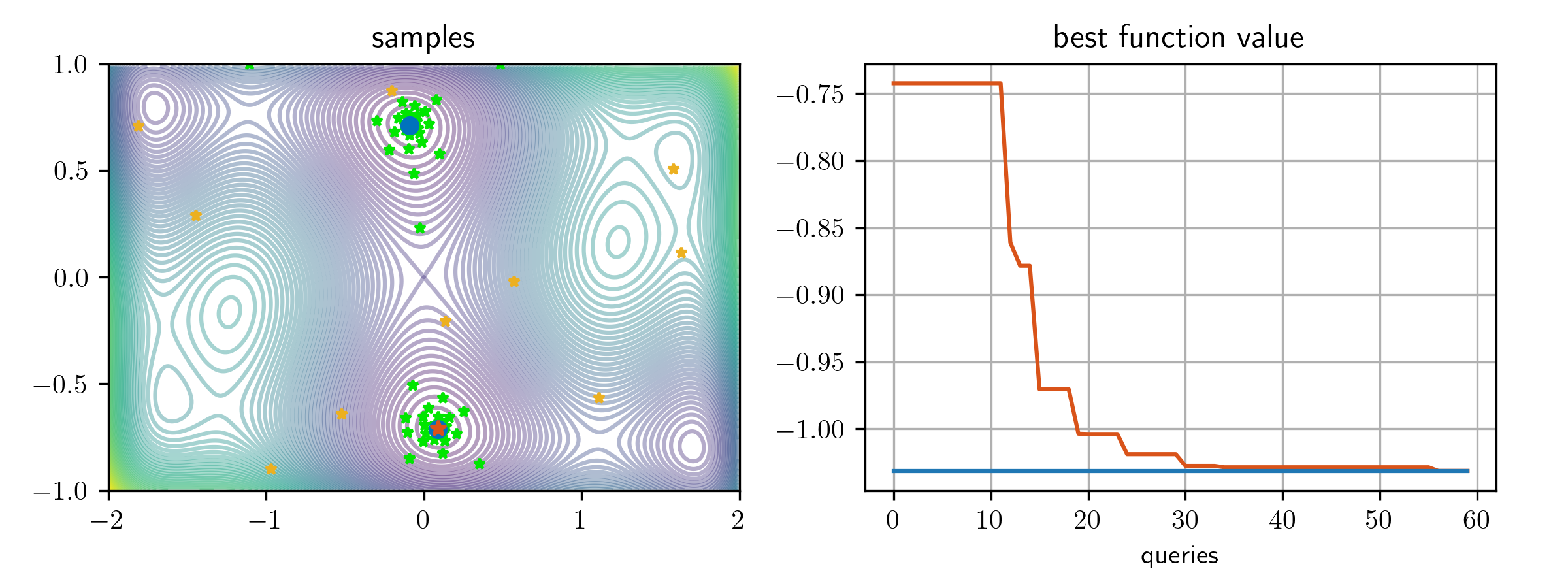
Here below is a plot of the samples xseq and best values fbest_seq found by GLIS:
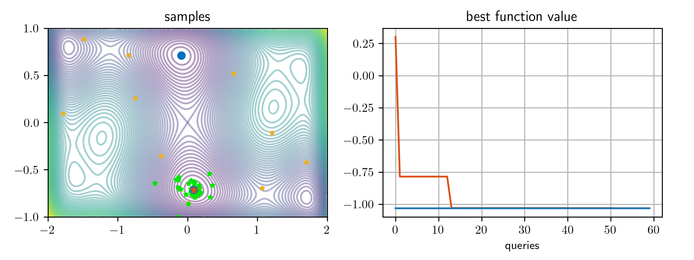
The yellow stars are the initial samples randomly generated by LHS, the green stars are the samples queried by GLIS during the active learning stage, the blue circles are the known global optimal solutions, and the red star is the optimizer identified by GLIS.
Next, we add linear constraints
    A = np.array([[1.6295, 1],[-1, 4.4553],[-4.3023, -1],[-5.6905, -12.1374],[17.6198, 1]])
    b = np.array([3.0786, 2.7417, -1.4909, 1, 32.5198])
    g = lambda x: np.array([x[0] ** 2 + (x[1] + 0.1) ** 2 - .5])
    prob = GLIS(bounds=(lb, ub), A=A, b=b, g=g, n_initial_random=10)
    xopt, fopt = prob.solve(fun, max_evals)
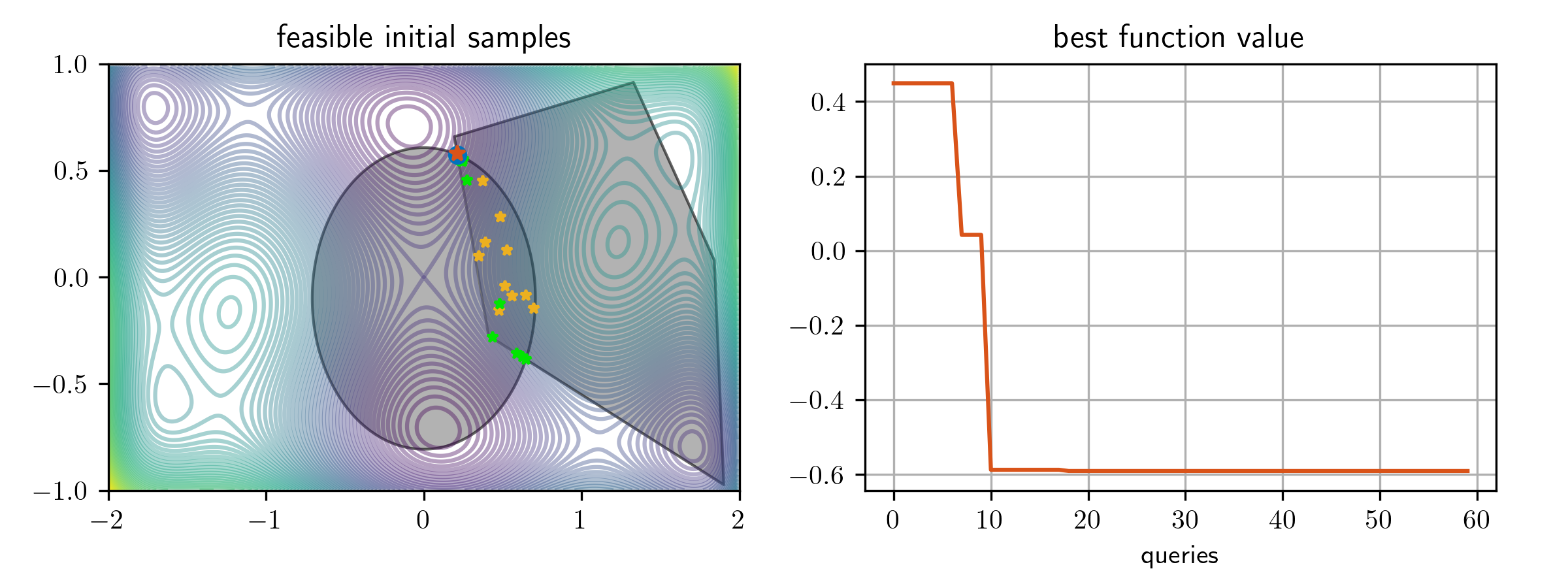
GLIS determines now a new optimizer within the given constraints:
In this case, the feasible region is the intersection of an ellipsoid and a polytope. Note that there is no requirement in GLIS that the constraints define a convex set.
More examples of numerical benchmark testing using GLIS can be found in the examples folder.
To solve a preference-based optimization problem with preference function lb ub use the following code:
from glis.solvers import GLISp
prob = GLISp(bounds=(lb, ub), n_initial_random=10)    # initialize GLISp object
xopt = prob.solve(pref_fun, max_prefs)                # solve problem
where pref_fun is the Python function implementing n_initial_random is the number of random samples taken at initialization, and max_prefs is the total allowed budget of preference queries collected from max_prefs+1 samples. The code returns the most preferred vector xopt found.
If additional preference queries can be done after running the optimization, the latter can be continued as follows:
xopt = prob.xbest         # current best sample found
x = prob.xnext            # next sample to compare to xopt
pref = pref_fun(x, xbest) # evaluate preference function
x = prob.update(pref)     # update GLISp object and get next sample to possibly query
xbest = prob.xbest        # updated optimizer
Alternatively, for a full step-by-step optimization without explicitly passing the function handle pref_fun to GLISp, use the following code structure to solve the problem step by step:
from glis.solvers import GLISp
prob = GLISp(bounds=(lb, ub), n_initial_random=10) # initialize GLISp object
xbest, x = prob.initialize()  # get first two random samples
for k in range(max_prefs):
    pref = pref_fun(x, xbest) # evaluate preference
    x = prob.update(pref)
    xbest = prob.xbest
xopt=xbest                    # final optimizer
A synthetic preference function pref_fun can be defined from a function fun as follows:
def pref_fun(x1,x2):
	# Synthetic preference function mapping (x1,x2) to {-1,0,1}
    tol = 1.e-3
    f1 = fun(x1)
    f2 = fun(x2)
    if f1 <= f2 - tol:
        pref = -1
    elif f1 >= f2 + tol:
        pref = 1
    else:
        pref = 0
return prefWe apply GLISp for optimizing the camel-six-humps function xopt = (-0.09967807, 0.71635488) (corresponding to $f(
Here below is a plot of the samples queried with bounds constraints:
and, with additional linear and nonlinear constraints:
More examples of numerical benchmark testing using GLISp can be found in the examples folder.
By default, GLIS/GLISp use the inverse quadratic RBF
with
use the following code:
from glis.rbf import gaussian
prob = GLIS(bounds=(lb, ub), n_initial_random=10, rbf=gaussian, rbf_epsil=3.0)
xopt, fopt = prob.solve(fun, max_evals)
The following RBFs are available in glis:
from glis.rbf import gaussian, inverse_quadratic, multiquadric, thin_plate_spline, linear, inverse_multi_quadricIn alternative to RBF functions, in GLIS we can use inverse distance weighting (IDW) surrogates:
prob = GLIS(bounds=(lb, ub), n_initial_random=10, rbf='IDW')
xopt, fopt = prob.solve(fun, max_evals)
Although IDW functions are simpler to evaluate, usually RBF surrogates perform better.
GLIS acquires a new sample
where
GLIS uses Particle Swarm Optimization (PSO) to determine the minimizer
By default, GLIS takes
To change the default values of the hyper-parameters
prob = GLIS(bounds=(lb, ub), alpha=0.5, delta=0.1)GLISp performs acquisition in a similar way than GLIS. The surrogate
GLISp also supports, in alternative, the acquisition based on the maximimization of the probability of improvement, as defined in [2]. This can be specified as follows:
prob = GLISp(bounds=(lb, ub), acquisition_method="prob_improvement")By default, acquisition_method = "surrogate".
The performance of GLISp can be usually improved by recalibrating
the RBF parameter
prob = GLISp(bounds=(lb, ub), RBFcalibrate=True, RBFcalibrationSteps=steps, thetas=thetas)where steps is an array of step indices at which recalibration must be performed, and thetas is the array of values of
To force the recalibration of the RBF at any time, use the command prob.rbf_recalibrate(), which computes the optimal value prob.theta of the scaling factor
As detailed in [3], GLIS/GLISp can handle unknown constraints on
prob = GLIS(bounds=(lb, ub), n_initial_random=13, has_unknown_constraints=True, has_satisfaction_fun=True)
xopt, fopt = prob.solve(fun, max_evals=50, unknown_constraint_fun=f1, satisfactory_fun=f2)
where f1 and f2 are the Python functions of f1 and f2 must be Boolean (True = feasible/satisfactory, False otherwise).
To solve the same problem in iterative form in GLIS, use the following example:
prob = GLIS(bounds=(lb, ub), n_initial_random=n_initial_random)
x = prob.initialize()
for k in range(max_evals):
    f = fun(x)
    fes = f1(x)
    sat = f2(x)
    x = prob.update(f, fes, sat)
xopt=prob.xopt
fopt=prob.fopt
A numerical benchmark with unknown constraints solved by GLIS can be found in file glis_unknown_constraints.py in the examples folder
while in GLISp:
prob = GLISp(bounds=(lb, ub), n_initial_random=n_initial_random, RBFcalibrate=True)
xbest, x = prob.initialize()  # get first two random samples
prob.eval_feas_sat(xbest, unknown_constraint_fun=f1, satisfactory_fun=f2)
for k in range(max_prefs):
    pref = pref_fun(x, xbest)  # evaluate preference
    prob.eval_feas_sat(x, unknown_constraint_fun=f1, satisfactory_fun=f2)
    x = prob.update(pref)
    xbest = prob.xbest
xopt = xbest
Numerical benchmarks with unknown constraints solved by C-GLISp (detailed in [3] ) can be found in glisp_unknown_constraints.py in the examples folder.
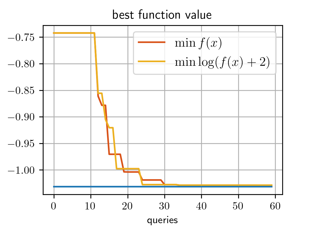
In GLIS, when the objective function has very large and very small values, it is possible to fit the surrogate of a nonlinear transformation of the objective rather the raw objective values. For example, in the camel-six-humps example we want to build the surrogate
prob = GLIS(bounds=(lb, ub), obj_transform=lambda f: np.log(f+2.), n_initial_random=10)
xopt, fopt = prob.solve(fun, max_evals)
Compare the best objective values found
Further options in executing GLIS/GLISp are detailed below:
svdtol tolerance used in SVD decomposition when fitting the RBF function.
shrink_range flag, if True the given bounds bounds are shrunk to the bounding box of the feasible constrained set
constraint_penalty penalty used to penalize the violation of the constraints
feasible_sampling flag, if True all the initial samples satisfy the constraints
scale_delta flag, scale
expected_max_evals expected maximum number of queries (defaulted to max_evals when using GLIS.solve().
display verbosity level: 0 = none (default).
PSOiters, PSOswarmsize, PSOminfunc: parameters used by the PSO solver from the pyswarm
package used by GLIS.
sepvalue (GLISp only): amount of separation
epsDeltaF (GLISp only): lower bound on the range of the surrogate function.
This package was coded by Alberto Bemporad and Mengjia Zhu. Marco Forgione and Dario Piga also contributed to the development of the package.
This software is distributed without any warranty. Please cite the above papers if you use this software.
@article{Bem20,
    author={A. Bemporad},
    title={Global optimization via inverse distance weighting and radial basis functions},
    journal={Computational Optimization and Applications},
    volume=77,
    pages={571--595},
    year=2020
}
@article{BP21,
    title={Active preference learning based on radial basis functions},
    author={A. Bemporad and D. Piga},
    journal={Machine Learning},
    volume=110,
    number=2,
    pages={417--448},
    year=2021
}
@article{ZPB22,
    author={M. Zhu and D. Piga and A. Bemporad},
    title={{C-GLISp}: Preference-Based Global Optimization under Unknown Constraints with Applications to Controller Calibration},
    journal={IEEE Transactions on Control Systems Technology},
    month=sep,
    volume=30,
    number=3,
    pages={2176--2187},
    year=2022
}
Apache 2.0
(C) 2019-2023 A. Bemporad, M. Zhu


